SHAP values for GBTs – intuition + how they work internally
This blog explores how Gradient Boosted Trees can be explained using PDP, ICE, and SHAP — with TreeSHAP making black-box models transparent and highly interpretable.
While training our ML models, we have access to amazing algorithms to help model our data to highest accuracy. But what happens to knowing why our model predicted a certain value or class? Most of the time... Its crickets
This blog takes you through that journey, starting with tree-based models, examining how they trade off bias and variance, and then pulling back the curtain with explainability techniques like PDP, ICE, and SHAP. Along the way, we’ll use a fitness dataset as our playground, highlighting not just performance metrics but also the subtle caveats that come with interpreting models.
1. From Decision Trees to Boosting
Decision Trees are the most natural starting point. A single tree is like a flowchart of yes/no rules, They are quick to train, easy to explain, but fragile. Sometimes they may remain shallow resulting in an underfit model, if too deep and it memorizes noise.
Random Forests improved on this by averaging across many trees grown on bootstrapped samples with randomized splits. The result: variance drops, predictions stabilize, and accuracy improves. In our dataset, Random Forests reached about 76% accuracy, the best of all.
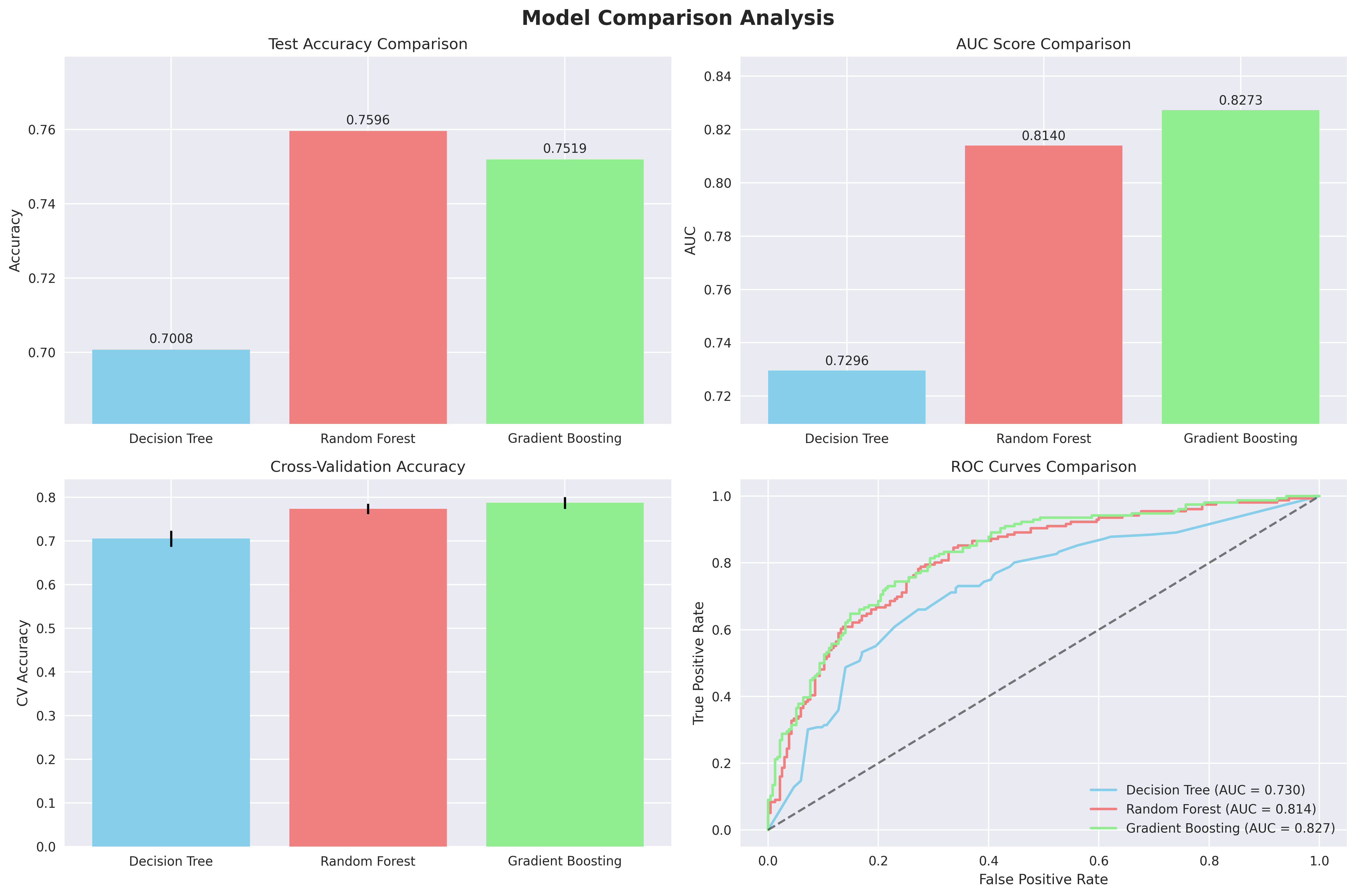
Gradient Boosted Trees take a different path. Instead of many independent trees, they grow trees sequentially, each one correcting the residual errors of the last. This iterative optimization often sharpens decision boundaries and reduces bias. Our boosted model landed at a similar accuracy (75%) but achieved a higher AUC (0.83 vs. 0.81), hence it was better at ranking who is likely to be fit.
So, the first lesson: bagging (Random Forests) calms variance, boosting attacks bias, and their relative performance depends on whether stability or fine-grained ranking matters more.
2. Looking Inside with PDP and ICE
Once we have models that predict fitness, the next question is: why? Traditional feature importance scores tell us which features are used often but not how they push predictions up or down. That’s where Partial Dependence Plots (PDP) and Individual Conditional Expectation (ICE) curves come in.
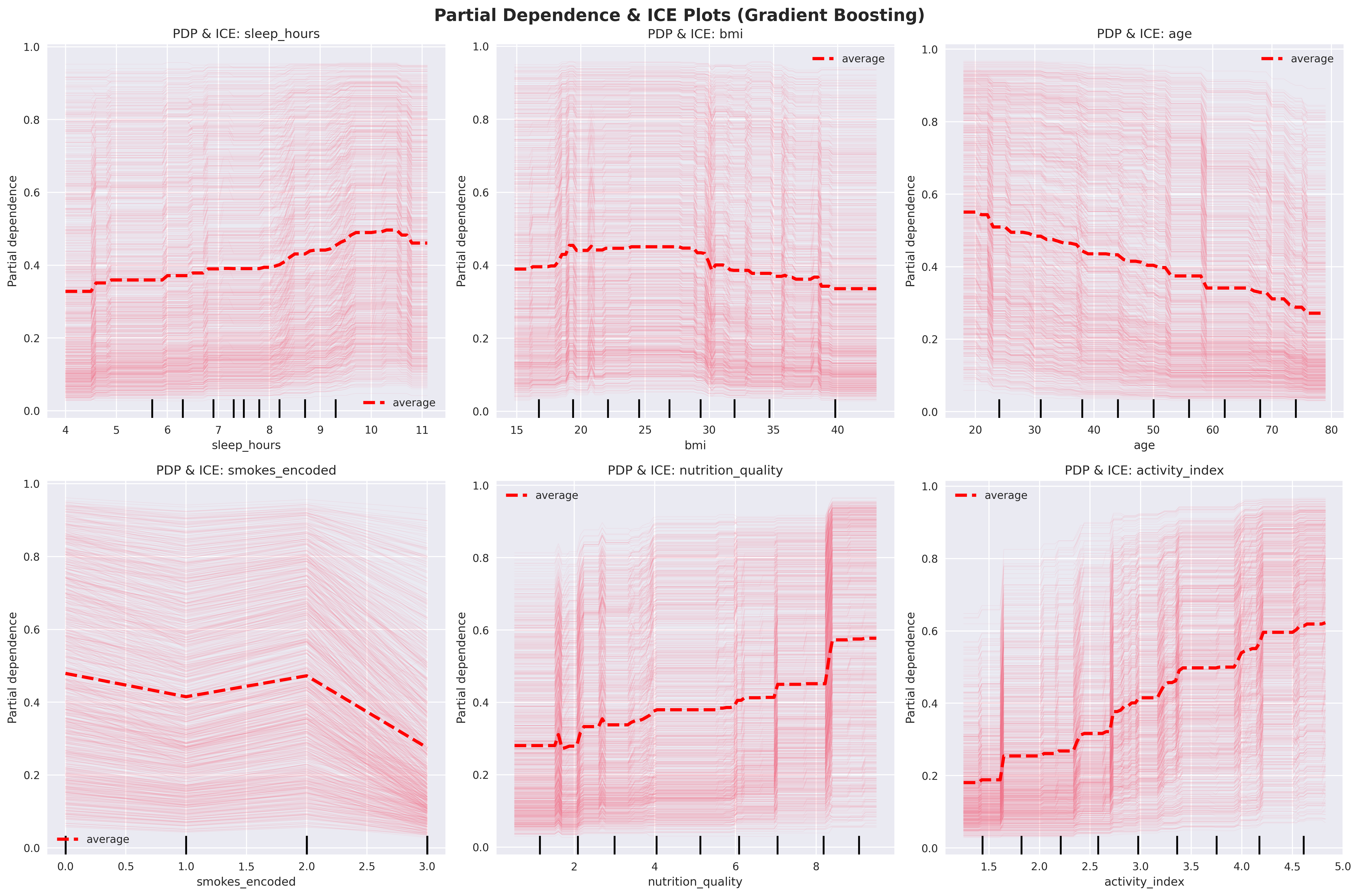
PDPs show the average effect of a feature by sweeping it across values while holding others fixed. In our case, sleep hours had a clear upward slope which can be interpreted as more rest = higher fitness probability. ICE plots take this further, drawing one line per individual. Here, heterogeneity surfaced: smokers of different ages showed very different curves.
But these methods have caveats. PDP assumes features are independent, which is shaky if, say, BMI, weight, and height are strongly correlated. ICE can overwhelm with noise in large datasets. And for categoricals, ordinal encoding (like smokes=0,1,2) can create misleading artificial orderings. One-hot encoding or SHAP handles these cases better.
3. Enter SHAP: From Averages to Explanations
While PDP and ICE offer useful intuition, they only sketch the picture. SHAP (SHapley Additive exPlanations) gives us the mathematical rigor of game theory. Think of each feature as a player and the model prediction as the payout. SHAP fairly divides credit among features by averaging their contributions across all possible coalitions.
This makes SHAP powerful at two levels:
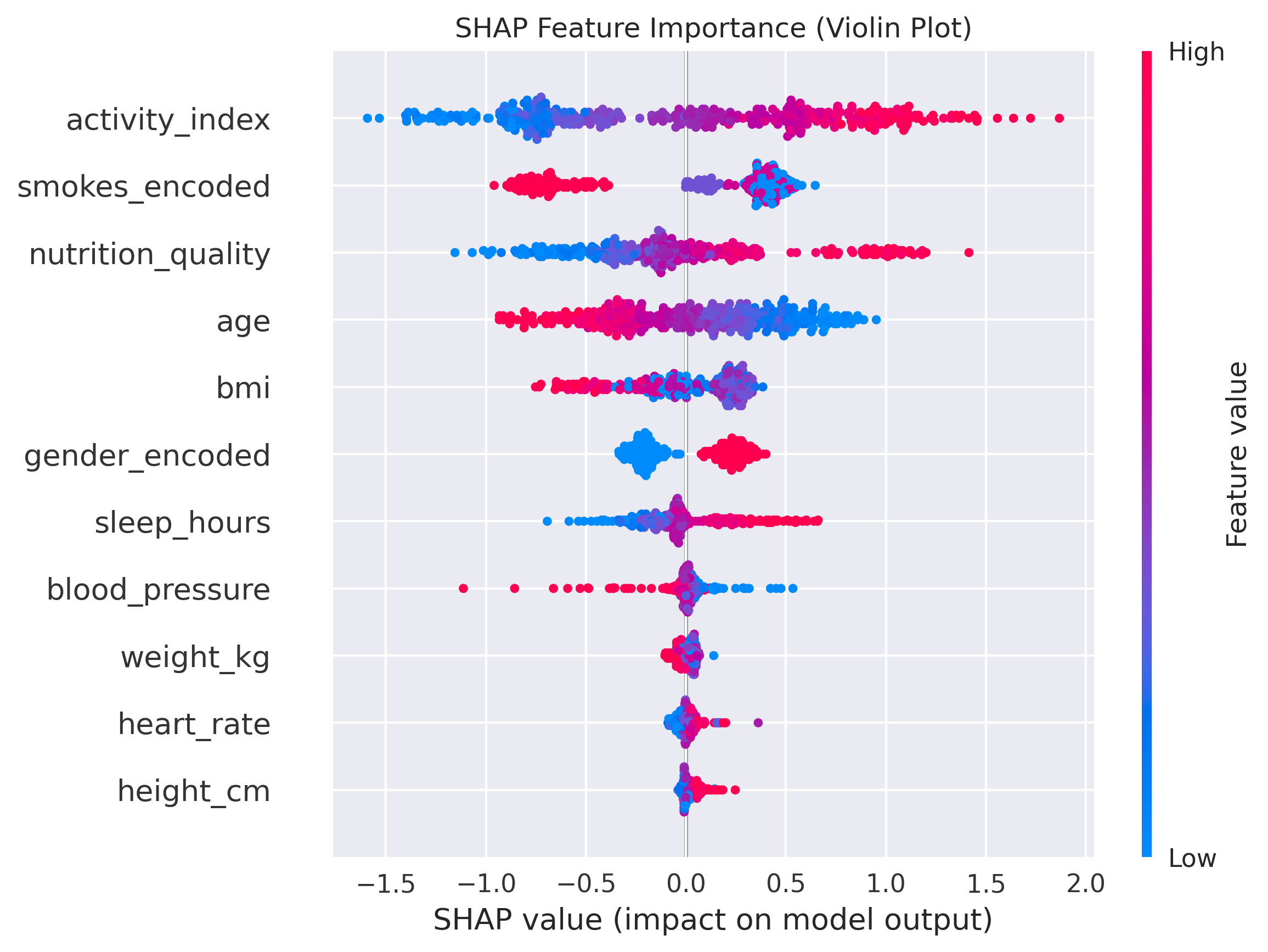
- Locally, it explains an individual prediction. For one subject in our dataset, SHAP showed that extra sleep added about +0.2 probability of being fit, while smoking subtracted –0.4.
- Globally, aggregating SHAP values revealed that Activity Index was the dominant factor overall, followed by Nutrition and Smoking habits.
Yet even SHAP has limits. Standard implementations assume features are independent; with correlated inputs, attributions may drift. Conditional SHAP variants or correlation-aware baselines are designed to address this.
4. TreeSHAP: Efficient Explanations for Ensembles
The original method for calculating Shapley values involves a combinatorial problem that quickly becomes intractable. To determine the importance of a single feature, you must consider all possible coalitions of features. A coalition is a subset of features used to make a prediction. The number of these subsets grows exponentially with the number of features, 2^M, where M is the number of features. For a model with just 20 features, this means considering over a million subsets, making the exact calculation computationally impossible for most datasets.
TreeSHAP overcomes this by leveraging the tree structure of the model. Instead of evaluating all possible feature combinations, it traces all possible paths down a decision tree. A key insight is that the order in which features are added to a coalition corresponds to a path through the tree. TreeSHAP can efficiently compute the expected marginal contribution of a feature by traversing the tree and summing up contributions at each split, weighted by the number of samples in that branch. It exploits the fact that for a given path, the contribution of a feature is determined by the difference in predictions at the nodes above and below the split that uses that feature. By doing this recursively for all paths and all trees in the ensemble, it calculates the exact SHAP value in polynomial time.
In practice, this means libraries like XGBoost and LightGBM let you extract SHAP attributions directly. In our fitness experiment, TreeSHAP produced global summary plots and local decision plots without prohibitive computation, turning what once felt like a black box into something transparent and verifiable.
Closing Thoughts
Our fitness dataset experiment highlights a broader truth about machine learning: raw accuracy is only half the story. Random Forests and Gradient Boosted Trees gave us competitive predictive performance, but the real value came when we dug into why the models behaved as they did.
PDP offered broad trends, ICE revealed individual variability, and SHAP — especially TreeSHAP — delivered a mathematically grounded explanation at both the local and global scale.