Introduction

Vector databases are one of the most popular and widely used systems in the tech industry. Their market was valued at ≈2.5 billion in 2024 and is projected to >3 billion in 2025. Over 70% of all organizations investing/implementing AI use vector databases for searching and embedding.

I have used vector databases in multiple use cases and projects. Be it RAG, searching and filtering documents or even feeding context to agents. After using multiple databases like FAISS, ChromaDB, Pinecone and pgvector, I was fascinated by vector databases and their internal workings.

Hence, I decided to implement one myself.

CapybaraDB, it is a lightweight vector database implementation, built from scratch in Python:

• It can perform semantic search using sentence-transformers for embeddings.
• It supports built-in token-based chunking.
• CUDA acceleration.
• Precision control (float32, float16, binary).
• .npz file storage for persistance.

What is a Vector Database?

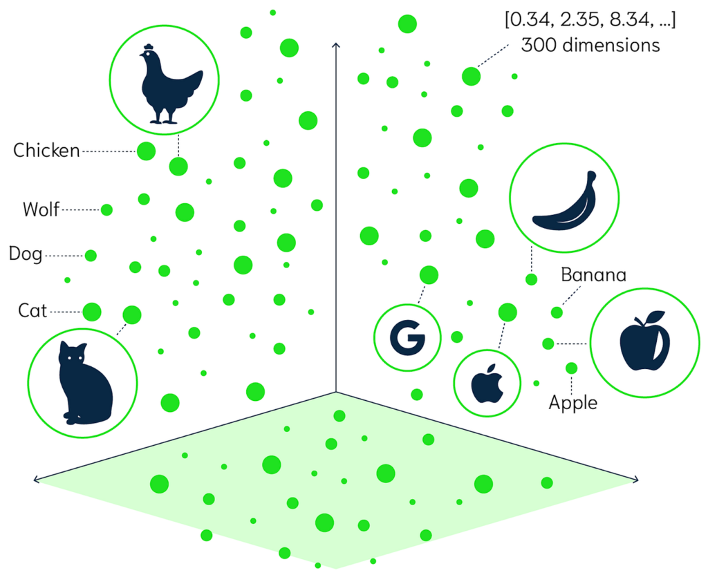
A vector database is a very special type of database which is very efficient in storing and searching dimensional vector embeddings. Embeddings are basically numerical representations of data like text, images, videos, audio, etc. In terms of structure, these embeddings are made up of array of floating point numbers representing the direction and magnitude of the generated vector.

A traditional database searches for exact match for the query entered, but vector databases find items by measuring the distance/difference between the query vector and embedded vectors inside the multidimensional space. Metrics like, euclidean distance or cosine similiarity can be used to measure distances between the vectors.

They're essential for modern AI applications including semantic search (finding meaning, not just keywords), recommendation systems, RAG (Retrieval Augmented Generation) for chatbots, image similarity search, and anomaly detection.

Popular examples include Pinecone, Weaviate, Milvus, Qdrant, and Chroma. They've become crucial infrastructure as AI applications need to search through millions of embeddings in milliseconds while maintaining accuracy.

Design Philosophy

1. Simplicity

   • A "toy" vector db implementation, aiming for minimal complexity
   • Straightforward APIs (add_document, search, get_document)
   • Minimal config to get started

2. Flexibilty

   • Utility support for multiple file formats
   • Configurable precision levels (float32, float16 and binary)
   • Choice to keep in-memory store or on disk
   • GPU support

3. Minimal dependencies

   • Core dependencies limited to essential libs
   • Lightweight footprint for prototyping and learning

4. Educational focus

   • Demonstrating fundamental vector database concepts

Metrics & Benchmarks

Indexing Performance

Data source: benchmark_results/indexing_performance.json

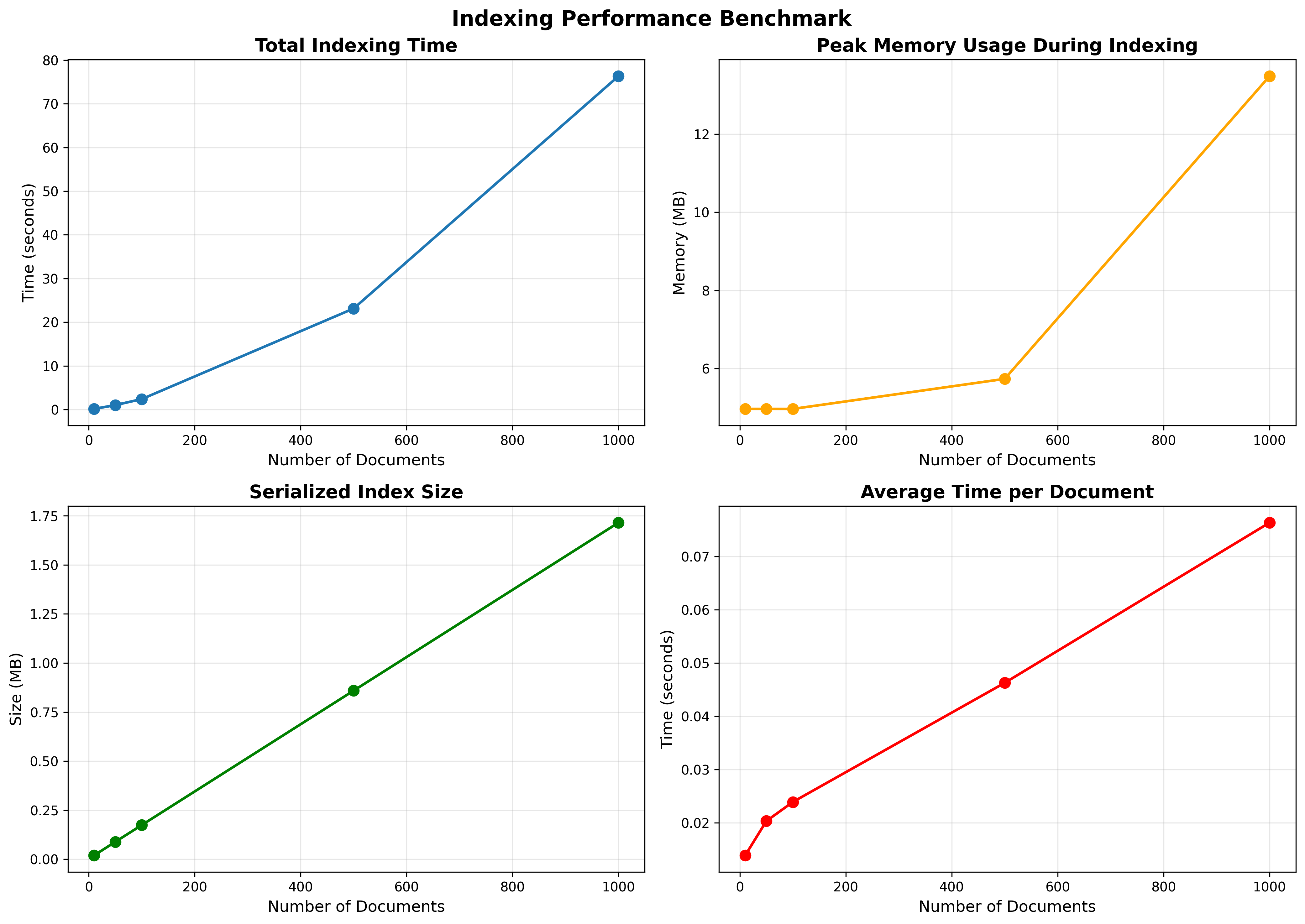
• Document counts tested: 10, 50, 100, 500, 1000
• Total times (s): 0.138, 1.015, 2.388, 23.126, 76.331
• Average time per doc (s): 0.0138, 0.0203, 0.0239, 0.0463, 0.0763
• Storage times remain small relative to embedding time even at 1k docs (≈0.122 s)
• Index size (MB): 0.020, 0.089, 0.174, 0.859, 1.715
• Peak memory (MB): ~2.2–65.4 across scales

Key takeaways:

• Embedding dominates total indexing time. Storage overhead is negligible in comparison.
• Linear growth with dataset size; average time per document rises as batches get larger and memory pressure appears.
• Index size scales linearly and remains compact for thousands of chunks.

Refer to benchmark_results/indexing_performance.png for the trend lines and indexing_performance_breakdown.png for stacked time components.

Query Performance

Data source: benchmark_results/query_performance.json

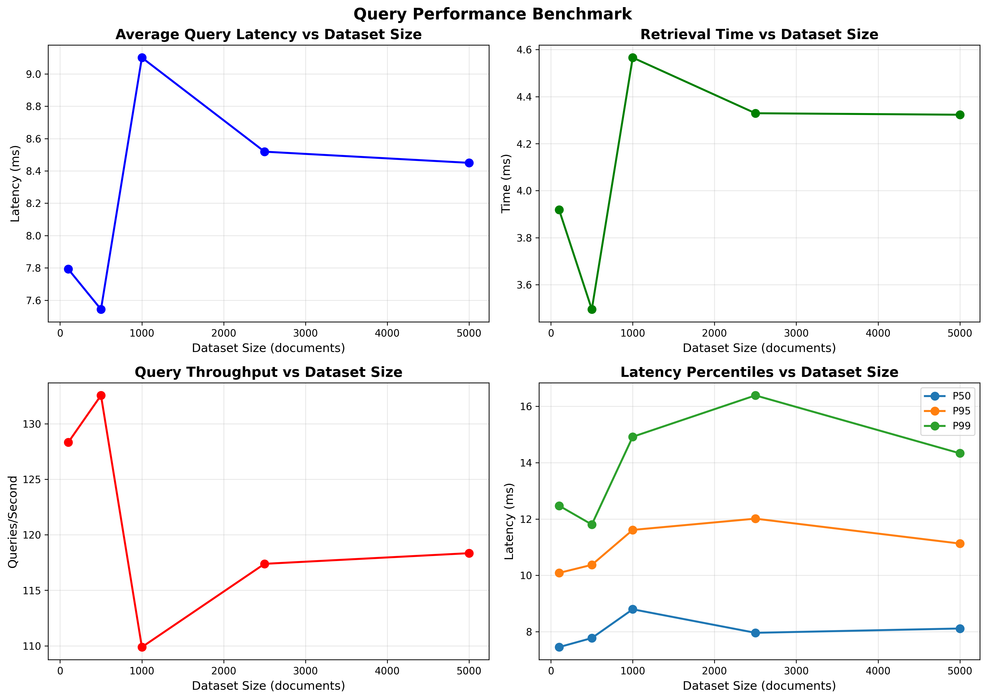
• Dataset sizes tested: 100, 500, 1000, 2500, 5000
• Average query latency (ms): 7.79, 7.54, 9.10, 8.52, 8.45
• Throughput (qps): 128.3, 132.6, 109.9, 117.4, 118.3
• p50 latency (ms): 7.45–8.79
• p95 latency (ms): 10.09–12.01
• p99 latency (ms): 11.80–16.39
• Breakdown (avg):
  • Embedding time (ms): ~3.87–4.53
  • Retrieval time (ms): ~3.50–4.57

Observations:

• Latency remains stable and low (≈7–9 ms on average) from 100 to 5000 vectors for top-k search, reflecting efficient vectorized exact search.
• Throughput remains >100 qps at all tested sizes.
• The split between query embedding and retrieval remains balanced; both contribute roughly half of total latency.
• Note: one anomalous value appears in min_latency_ms at 500 (-524.27 ms). This is a measurement artifact and should be ignored; distributional statistics (p50/p95/p99) are consistent and reliable.

Charts: benchmark_results/query_performance.png and query_performance_breakdown.png visualize latency distributions and the embedding vs retrieval split.

Retrieval Quality (Synthetic)

Data source: benchmark_results/retrieval_quality_synthetic.json

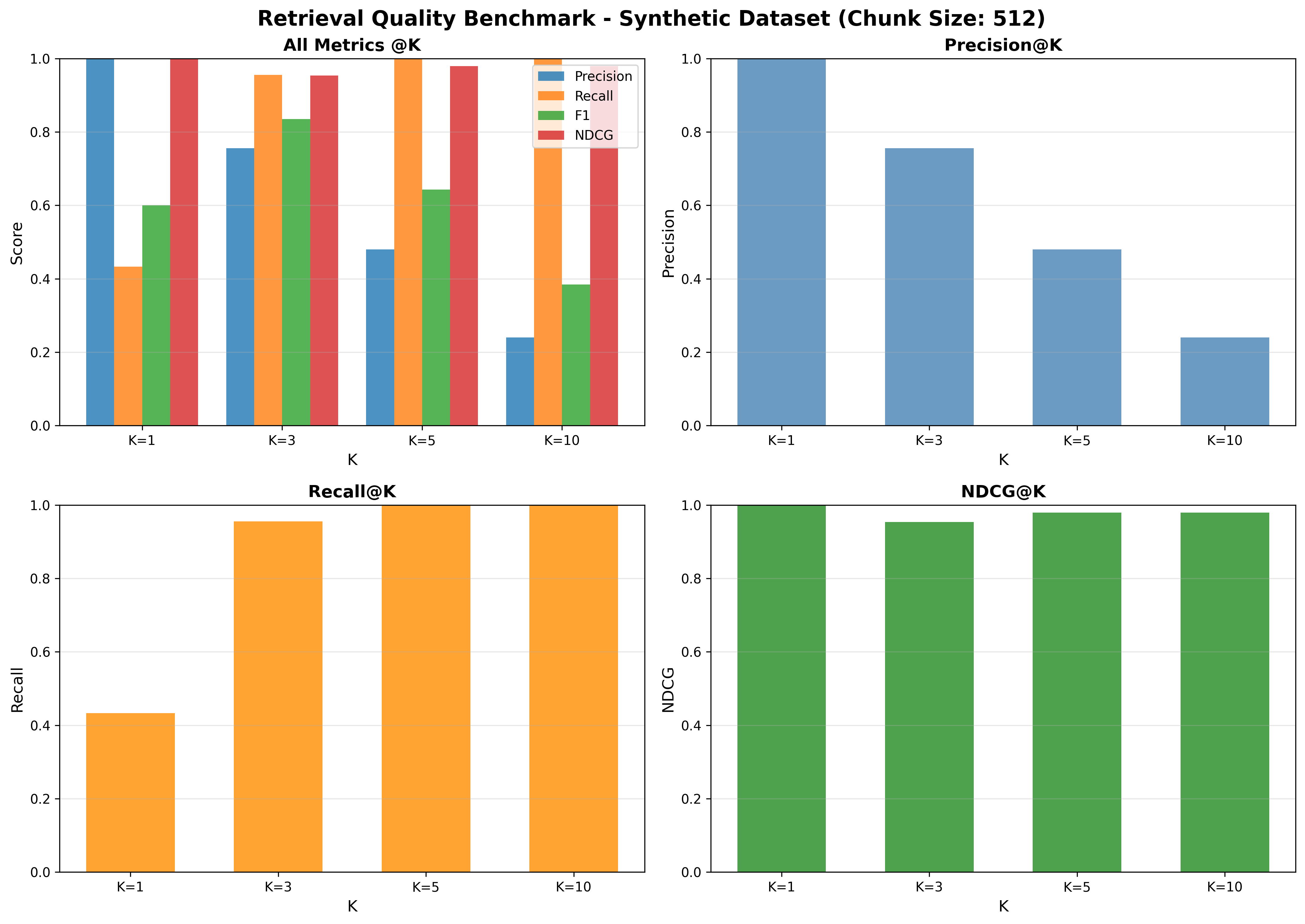
Configuration:

• Dataset: Synthetic
• Chunk size: 512

Quality metrics:

• Precision@k: P@1=1.00, P@3≈0.756, P@5≈0.480, P@10≈0.240
• Recall@k: R@1≈0.433, R@3≈0.956, R@5=1.00, R@10=1.00
• F1@k: F1@1=0.60, F1@3≈0.836, F1@5≈0.643, F1@10≈0.385
• nDCG@k: nDCG@1=1.00, nDCG@3≈0.954, nDCG@5≈0.979, nDCG@10≈0.979

Interpretation:

• Very strong early precision (P@1=1.0) and nDCG across cutoffs indicate effective ranking of the most relevant content.
• Near-perfect recall by k=5 shows top-5 captures essentially all relevant items.

See benchmark_results/retrieval_quality_synthetic.png for the quality curves.

Disclaimer ⚠️: The documents in the dataset used here are relatively short (typically well under 512 tokens).
As a result, a chunk size of 512 effectively corresponds to document-level embeddings — each document was indexed as a single vector.
While this setup is sufficient for small-scale or toy benchmarks, it may not generalize to longer documents where sub-document (passage-level) chunking becomes necessary for finer-grained retrieval.
Future evaluations will include experiments with smaller chunk sizes (e.g., 128–256) and longer document corpora to assess chunk-level retrieval effects.

What These Results Mean from a Perspective of A "Toy Database"

• Small to medium collections (≤10k chunks): exact search is fast, simple, and accurate.
• Low latency: median ≈7–9 ms per query with >100 qps throughput in benchmarks.
• Strong quality: excellent early precision and recall on the synthetic task with coherent chunking.
• Scales linearly: indexing and index size grow linearly; storage overhead is minimal compared to embedding time.

Core Architecture

1. BaseIndex

The main in-memory (temp) data store of CapybaraDB is the BaseIndex class, a data structure that holds:

class BaseIndex:
    documents: Dict[str, str]           # doc_id -> full document text
    chunks: Dict[str, Dict[str, str]]   # chunk_id -> {text, doc_id}
    vectors: Optional[torch.Tensor]     # All chunk embeddings
    chunk_ids: List[str]                # Order-preserving chunk IDs
    total_chunks: int
    total_documents: int
    embedding_dim: Optional[int]

This design keeps documents and their chunks separate while maintaining relationships through IDs. Why this separation? It allows us to:

• Return full documents when retrieving search results
• Track which chunk belongs to which document
• Maintain metadata without duplicating data

2. Index

The Index class extends BaseIndex with persistence:

class Index(BaseIndex):
    def __init__(self, storage_path: Optional[Path] = None):
        super().__init__()
        self.storage = Storage(storage_path)

This is where of auto-loading happens. When you create an Index, it checks if a persisted version exists and loads it automatically. This is of-course optional, if no path is provided, the db is kept in-memory.

3. CapybaraDB: The Main Interface

The CapybaraDB class which exposes the API:

class CapybaraDB:
    def __init__(
        self,
        collection: Optional[str] = None,
        chunking: bool = False,
        chunk_size: int = 512,
        precision: Literal["binary", "float16", "float32"] = "float32",
        device: Literal["cpu", "cuda"] = "cpu",
    ):

You can create multiple collections, control chunking, adjust precision, and choose your compute device.

Embeddings

1. Architecture

CapybaraDB uses sentence-transformers/all-MiniLM-L6-v2, a lightweight transformer model that converts text into 384-dimensional vectors.

class EmbeddingModel:
    def __init__(
        self,
        precision: Literal["binary", "float16", "float32"] = "float32",
        device: Literal["cpu", "cuda"] = "cpu",
    ):
        self.model_name = "sentence-transformers/all-MiniLM-L6-v2"
        self.tokenizer = AutoTokenizer.from_pretrained(self.model_name)
        self.model = AutoModel.from_pretrained(self.model_name).to(device)

The model is initialized once and reused for all embeddings, keeping operations fast and memory-efficient.

2. The Embedding Process

When you call embed() on a document, here's what happens:

def embed(self, documents: Union[str, List[str]]) -> torch.Tensor:
    encoded_documents = self.tokenizer(
        documents, padding=True, truncation=True, return_tensors="pt"
    )
    
    with torch.no_grad():
        model_output = self.model(**encoded_documents)
    
    sentence_embeddings = self._mean_pooling(
        model_output, encoded_documents["attention_mask"]
    )
    sentence_embeddings = F.normalize(sentence_embeddings, p=2, dim=1)

1. Tokenization: Using tiktoken package and cl100kbase token encoding the chunks are tokenized
2. Generation: Production of context-aware representations for each position
3. Normalization: L2 norm to convert all vectors to unit length for accurate retrieval

3. Precision Modes

CapybaraDB supports three precision modes:

Float32 (default): Full precision, highest accuracy

Float16: Half precision, ~50% memory savings, minimal accuracy loss

Binary: Each dimension becomes 0 or 1, resulting in memory savings. The embedding process converts values > 0 to 1.0:

if self.precision == "binary":
    sentence_embeddings = (sentence_embeddings > 0).float()

Binary embeddings use a scaled dot product during search to compensate for information loss.

Document Processing Pipeline

Adding a Document

When you add a document, here's the full journey:

def add_document(self, text: str, doc_id: Optional[str] = None) -> str:
    if doc_id is None:
        doc_id = str(uuid.uuid4())
    
    self.index.documents[doc_id] = text
    self.index.total_documents += 1

Step 1: ID Generation

If no ID is provided, we generate a UUID. This ensures every document is uniquely identifiable.

Step 2: Chunking (Optional)

If chunking is enabled, the document is split using token-based chunking:

if self.chunking:
    enc = tiktoken.get_encoding("cl100k_base")
    token_ids = enc.encode(text)
    chunks = []
    for i in range(0, len(token_ids), self.chunk_size):
        tok_chunk = token_ids[i : i + self.chunk_size]
        chunk_text = enc.decode(tok_chunk)
        chunks.append(chunk_text)

Why token-based chunking instead of character-based?

• Respects word boundaries
• Considers tokenizer structure
• Produces more semantically coherent chunks
• Works better with the embedding model

Step 3: Create Chunks

Each chunk gets its own UUID and is stored with metadata:

for chunk in chunks:
    chunk_id = str(uuid.uuid4())
    self.index.chunks[chunk_id] = {"text": chunk, "doc_id": doc_id}
    chunk_ids.append(chunk_id)
    self.index.total_chunks += 1

Step 4: Generate Embeddings

All chunks are embedded in one batch:

chunk_texts = [self.index.chunks[cid]["text"] for cid in chunk_ids]
chunk_embeddings = self.model.embed(chunk_texts)

Batch processing is key to performance. Embedding 100 chunks together is much faster than 100 individual embeddings.

Step 5: Append to Vector Store

This is where the vectors are added to the index:

if self.index.vectors is None:
    self.index.vectors = chunk_embeddings
    self.index.chunk_ids = chunk_ids
    self.index.embedding_dim = chunk_embeddings.size(1)
else:
    self.index.vectors = torch.cat(
        [self.index.vectors, chunk_embeddings], dim=0
    )
    self.index.chunk_ids.extend(chunk_ids)

The first document creates the tensor. Subsequent documents are concatenated along the batch dimension.

Step 6: Persistence

If not in-memory mode, the index is saved immediately:

if not self.index.storage.in_memory:
    self.index.save()

This means you can add documents and they're persisted incrementally—no manual save needed!

The Search Engine

The Search Process

Here's how search works end-to-end:

def search(self, query: str, top_k: int = 5):
    if self.index.vectors is None:
        return []
    
    self.index.ensure_vectors_on_device(target_device)
    indices, scores = self.model.search(query, self.index.vectors, top_k)
    
    results = []
    for idx, score in zip(indices.tolist(), scores.tolist()):
        chunk_id = self.index.chunk_ids[idx]
        chunk_info = self.index.chunks[chunk_id]
        doc_id = chunk_info["doc_id"]
        
        results.append({
            "doc_id": doc_id,
            "chunk_id": chunk_id,
            "text": chunk_info["text"],
            "score": score,
            "document": self.index.documents[doc_id],
        })
    
    return results

Step 1: Query Embedding

The query text is embedded using the same model:

def search(self, query: str, embeddings: torch.Tensor, top_k: int):
    query_embedding = self.embed(query)

Step 2: Similarity Computation

The similarity between query and all stored vectors is computed:

if self.precision == "binary":
    similarities = torch.matmul(
        embeddings.float(), 
        query_embedding.t().float()
    ) / query_embedding.size(1)
else:
    similarities = torch.matmul(embeddings, query_embedding.t())

For each query, the system computes similarity with all stored vectors. In binary precision, it performs a dot product between 0/1 vectors, scaled by the embedding dimension—yielding the fraction of matching active bits. In float precision, normalized embeddings use standard cosine similarity via matrix multiplication with the query embedding.

Step 3: Top-K Selection

We use torch.topk to find the most similar vectors:

scores, indices = torch.topk(
    similarities.squeeze(),
    min(top_k, embeddings.size(0))
)

Step 4: Result Assembly

For each result, we reconstruct the full context by:

1. Looking up the chunk text
2. Finding the parent document ID
3. Retrieving the full document

This gives you both the specific chunk that matched and the full document context.

Storage and Persistence

The Storage Layer

The Storage class handles persistence with NumPy's compressed NPZ format:

def save(self, index) -> None:
    data = {
        "vectors": index.vectors.cpu().numpy(),
        "chunk_ids": np.array(index.chunk_ids),
        "chunk_texts": np.array([index.chunks[cid]["text"] for cid in index.chunk_ids]),
        "chunk_doc_ids": np.array([index.chunks[cid]["doc_id"] for cid in index.chunk_ids]),
        "doc_ids": np.array(list(index.documents.keys())),
        "doc_texts": np.array(list(index.documents.values())),
        "total_chunks": index.total_chunks,
        "total_documents": index.total_documents,
        "embedding_dim": index.embedding_dim or 0,
    }
    
    np.savez_compressed(self.file_path, **data)

Why NPZ?

• Compressed by default (saves space)
• Efficient binary format
• Handles large arrays well
• Cross-platform and language-agnostic

In-Memory vs Persistent

CapybaraDB supports two modes:

In-Memory: No file path specified. Data stays in RAM, lost on exit.

Persistent: File path specified. Data is saved to disk after each add_document() call.

This dual-mode design enables both temporary experiments (in-memory) and production use (persistent).

Putting It All Together

Example: Simple Document Search

from capybaradb.main import CapybaraDB
 
# Initialize
db = CapybaraDB(
    collection="research_papers",
    chunking=True,
    chunk_size=512,
    device="cuda"
)
 
# Add documents
doc1_id = db.add_document("Machine learning is transforming NLP...")
doc2_id = db.add_document("Deep neural networks excel at image recognition...")
 
# Search
results = db.search("artificial intelligence", top_k=2)
 
# Use results
for result in results:
    print(f"Score: {result['score']:.4f}")
    print(f"Matched text: {result['text'][:100]}...")
    print(f"Full document: {result['document']}")
    print("---")

Conclusion

Implementation: GitHub

This implementation of CapybaraDB was purely for education purposes and my own learning. I had a great time figuring out the nitty-gritty details behind vector databases and will definitely take on more challenging implementations in the future.