Training a Mixture-of-Experts Router
I was curious about MoEs, so I implemented and tested one.

Introduction
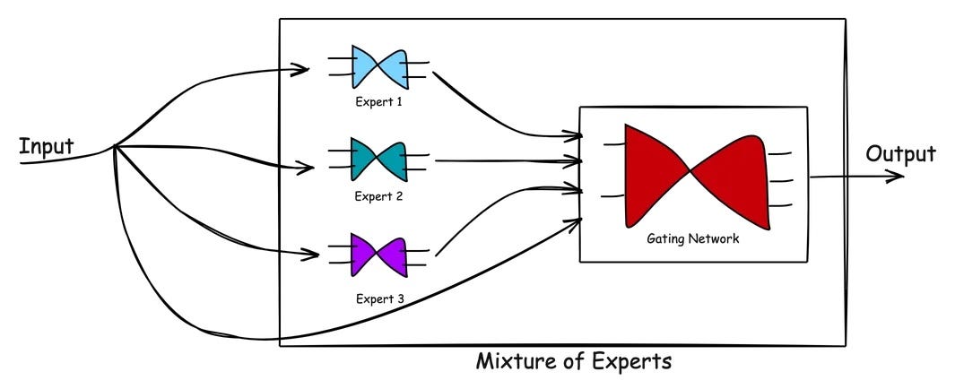
Since Deepseek-MoE introduced the MoE architecture, I was aware of it and saw it's adoption across the open source and proprietary model providers. But I never tried to understand the idea deeper. The idea that you can expand a model’s capacity without sending every token through a huge feed-forward block felt very interesting.
I tried to write the whole thing myself, from data loading and tokenization to a GPT-style transformer with optional MoE layers. This included the dataset pipeline, transformer blocks, routing logic, expert modules, and a training loop that tracked timing, throughput, losses, and expert usage.
This blog walks through what I learned, how each component fits together, and the results that stood out, with the hope that these insights help anyone curious about MoE models or planning to build one.
Project Plan
Before writing any code, I outlined the system I wanted. I needed a modular setup that let me swap dense layers for MoE layers, try different routing strategies, and run controlled comparisons without constant rewrites. That meant keeping data, model, MoE components, and training logic cleanly separated.
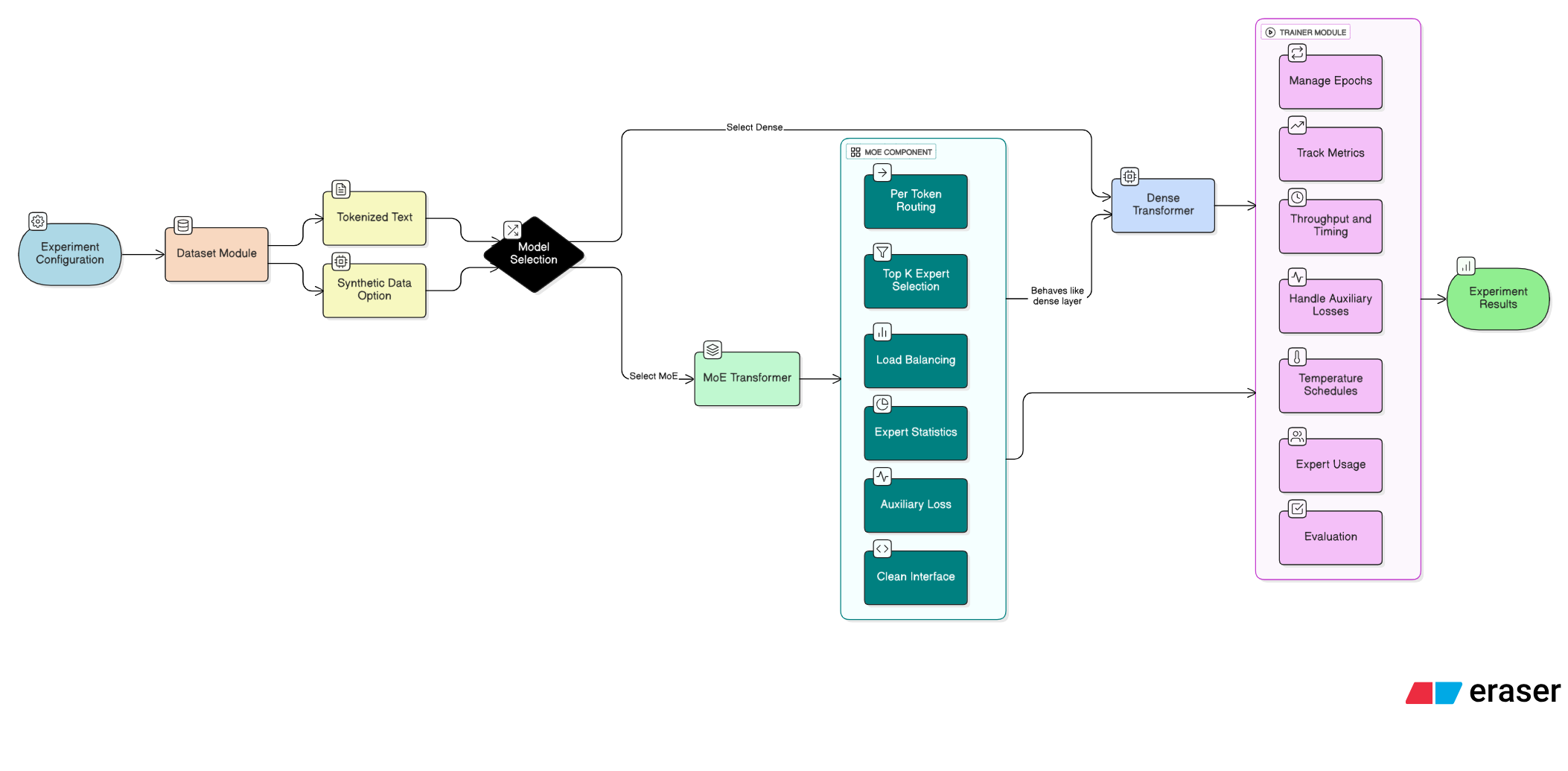
I began with the dataset pipeline. A steady source of tokenized text is essential for any language model experiment, and I wanted the option to fall back to synthetic data. After that, I focused on the model architecture. I planned to build a small GPT-style transformer first, since it provided a stable baseline and a familiar structure to extend with MoE layers. The goal was to keep the dense path intact while making the MoE path a drop-in replacement so both versions could be compared under identical conditions.
Next came the MoE module, which required the most iteration. I wanted per-token routing, top k selection, load balancing, and expert statistics without creating a messy forward pass. I mapped out how the router, experts, and auxiliary loss would interact and built an interface that let transformer blocks treat dense and MoE layers the same.
The final piece was the training loop. I needed detailed metrics: throughput, timing, auxiliary losses, temperature schedules, and expert usage. The Trainer class would handle epochs, collect metrics, and coordinate evaluation so experiments remained consistent.
With the components defined, the plan was straightforward: build the dataset module, implement the transformer, add the MoE layer, wire everything in the Trainer, and run dense and MoE configurations under a shared framework.
Implementation
Once the plan was set, the next step was turning each idea into a working module. I wanted the codebase to feel like a compact training stack with clear boundaries. That shaped how the transformer, MoE layer, and Trainer were built.
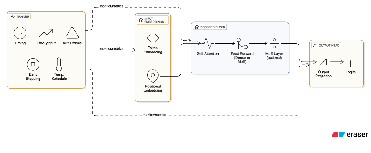
The transformer came first, following a standard GPT-style decoder with token embeddings, positional embeddings, a stack of self-attention blocks, and a final projection. The key feature was a pluggable feed-forward sublayer. If a layer index matched an MoE position, the dense FFN was swapped for an MoE layer through a shared interface. This made it easy to alternate between dense and sparse configurations without altering the architecture.
The MoE layer required the most careful engineering. Routing occurs per token, so the implementation flattens batch and sequence dimensions, applies a linear router, then uses a temperature scaled softmax to produce expert probabilities. Tokens pick top experts, pass through identical feed-forward experts, and are recombined with routing weights. The layer also tracks usage, probabilities, and entropy, which was crucial for spotting imbalance and specialization patterns.
With the model ready, the Trainer handled timing, throughput, auxiliary losses, and temperature schedules. It recorded detailed metrics, measured forward and backward phases separately, and supported early stopping. Together, these components formed a focused environment for comparing dense and MoE models and revealing their trade-offs.
Dataset
For these experiments I needed a dataset that was structured enough to reveal real modeling behavior yet small enough for fast iteration. WikiText-2 fit well. It contains high-quality English text from Wikipedia, offering natural sentence structures, topic shifts, and long-range dependencies that make model behavior easy to inspect.
I kept the raw text but used a custom tokenization pipeline instead of the original large vocabulary. I mapped everything into a fixed vocabulary of 10000 tokens. This kept the embedding matrix small and made the model lighter, while also shifting the dataset’s statistics. A smaller vocabulary increases sequence length due to more subword splits and raises the frequency of common tokens. That steeper distribution created clearer patterns early in training and made capacity differences between dense and MoE variants easier to observe.
The dataset is stored in Parquet format and loaded with Polars. After tokenization, it produces about 2.1 million training tokens and about 217000 validation tokens. These totals stay similar after remapping, although some lines become longer and the token distribution grows more concentrated.
A streaming dataset slices training sequences with sliding windows, keeping memory use low and avoiding preprocessing. I also added a synthetic fallback for development. Overall, WikiText-2 with a 10000-token vocabulary offered a realistic and efficient environment for comparing dense and MoE models.
MoE vs Dense: Experiment Results and Recommendations
TL;DR
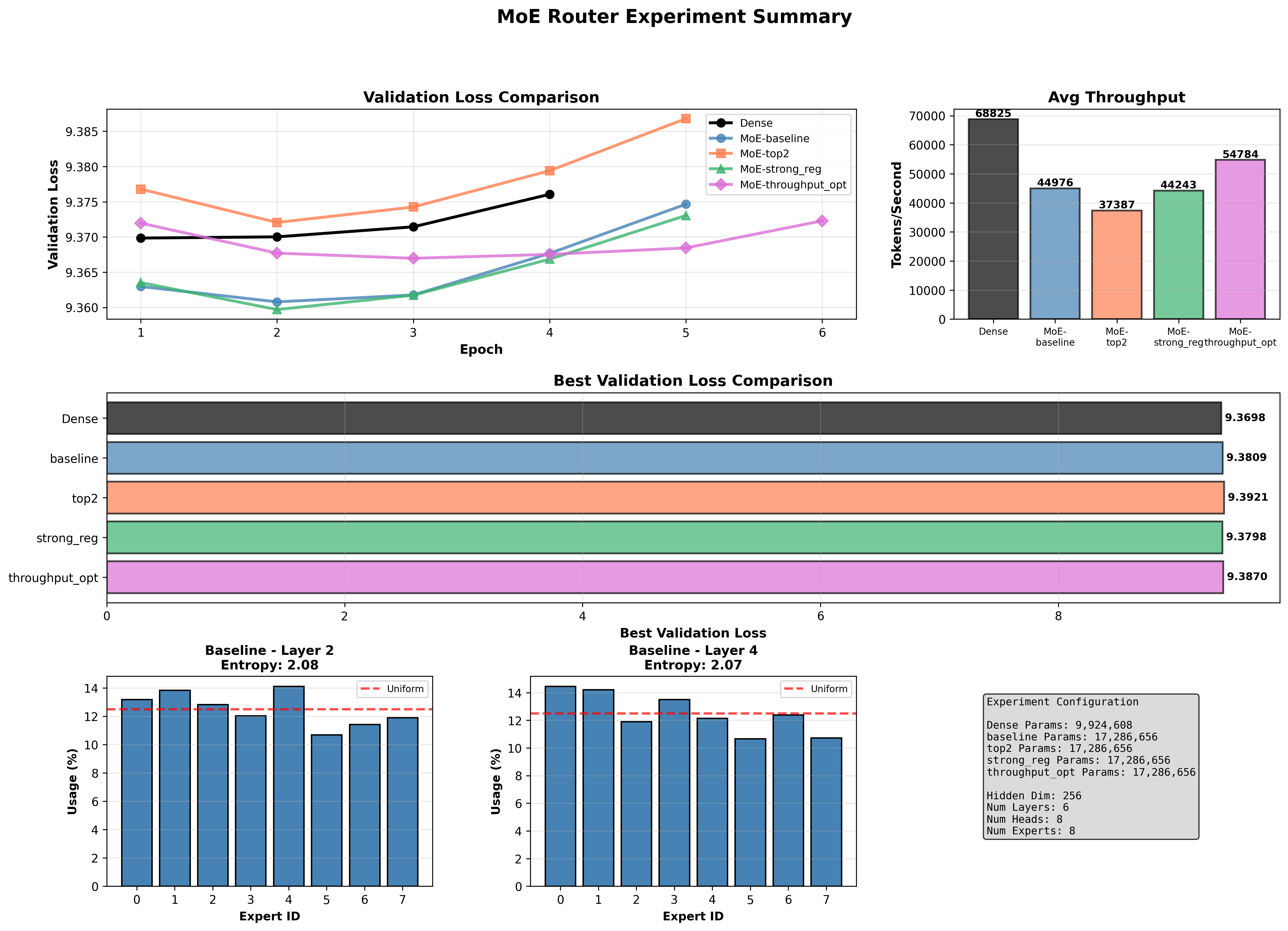
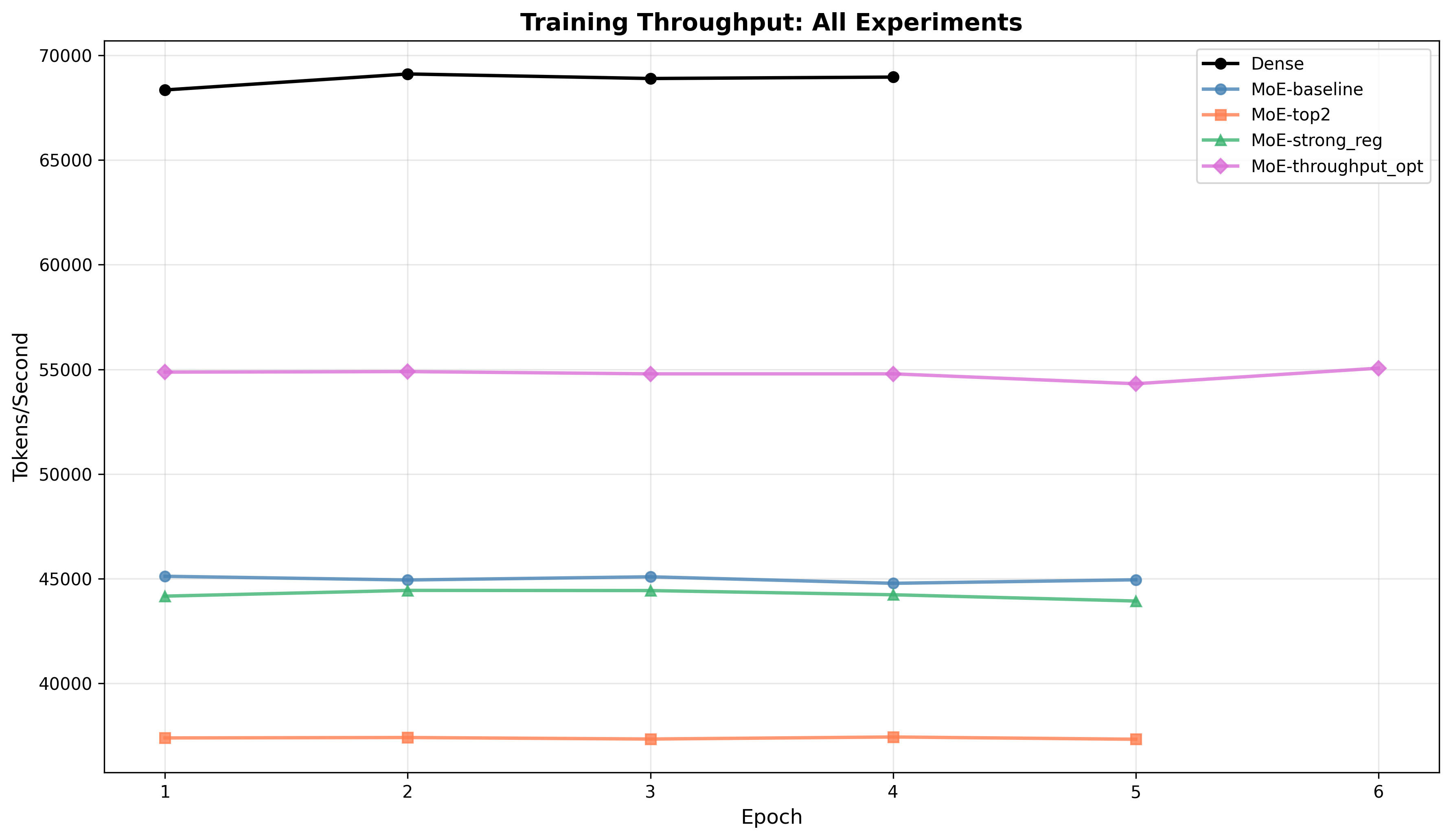
- The dense model achieved the best validation loss and the highest training throughput. It remains the strongest performer for this setup when evaluating generalization versus raw speed.
- Mixture-of-experts (MoE) variants increased model capacity (roughly 17.3M parameters vs 9.9M for the dense model) but introduced substantial runtime overhead, primarily in the backward pass. That overhead reduced tokens/sec compared with the dense baseline.
- Among MoE variants,
throughput_optsubstantially reduced backward cost compared with the other MoEs and delivered the best throughput among MoEs, but it did not match the dense model in tokens/sec or in best validation loss. top2reached the lowest training loss but the worst validation loss, suggesting overfitting or instability in gating/generalization.- Routing entropy and per-expert usage indicate reasonably balanced expert assignment across experiments, but layer- and experiment-level differences remain and may explain some of the generalization differences.
Key numbers (single-epoch timing, parameters, best validation loss, avg throughput)
| Model | Params | Best validation loss | Avg throughput (tokens/sec) | Forward (s) | Backward (s) | Optimizer (s) | Total per-epoch (s) |
|---|---|---|---|---|---|---|---|
| Dense | 9,924,608 | 9.3698 | 68,825 | 0.40 | 0.20 | 0.03 | 0.63 |
| MoE-baseline | 17,286,656 | 9.3809 | 44,976 | 0.75 | 1.17 | 0.05 | 1.97 |
| MoE-top2 | 17,286,656 | 9.3921 | 37,387 | 0.90 | 1.47 | 0.05 | 2.42 |
| MoE-strong_reg | 17,286,656 | 9.3798 | 44,243 | 0.76 | 1.19 | 0.05 | 2.00 |
| MoE-throughput_opt | 17,286,656 | 9.3870 | 54,784 | 0.56 | 0.96 | 0.03 | 1.55 |
Training and validation dynamics
-
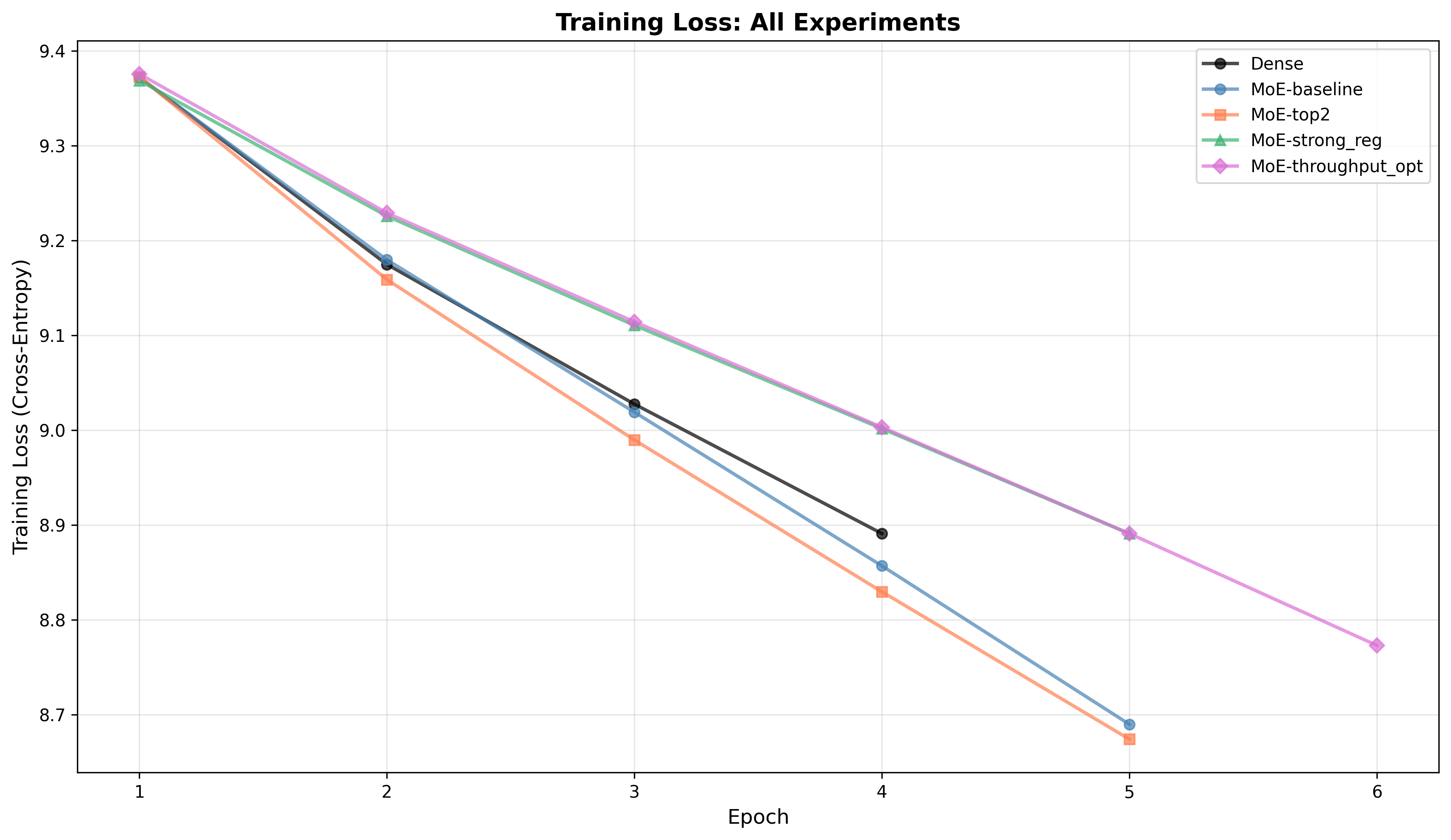
Training loss: All variants show steadily decreasing training loss.
MoE-top2reaches the lowest training loss across epochs, indicating higher capacity or faster training fit. -
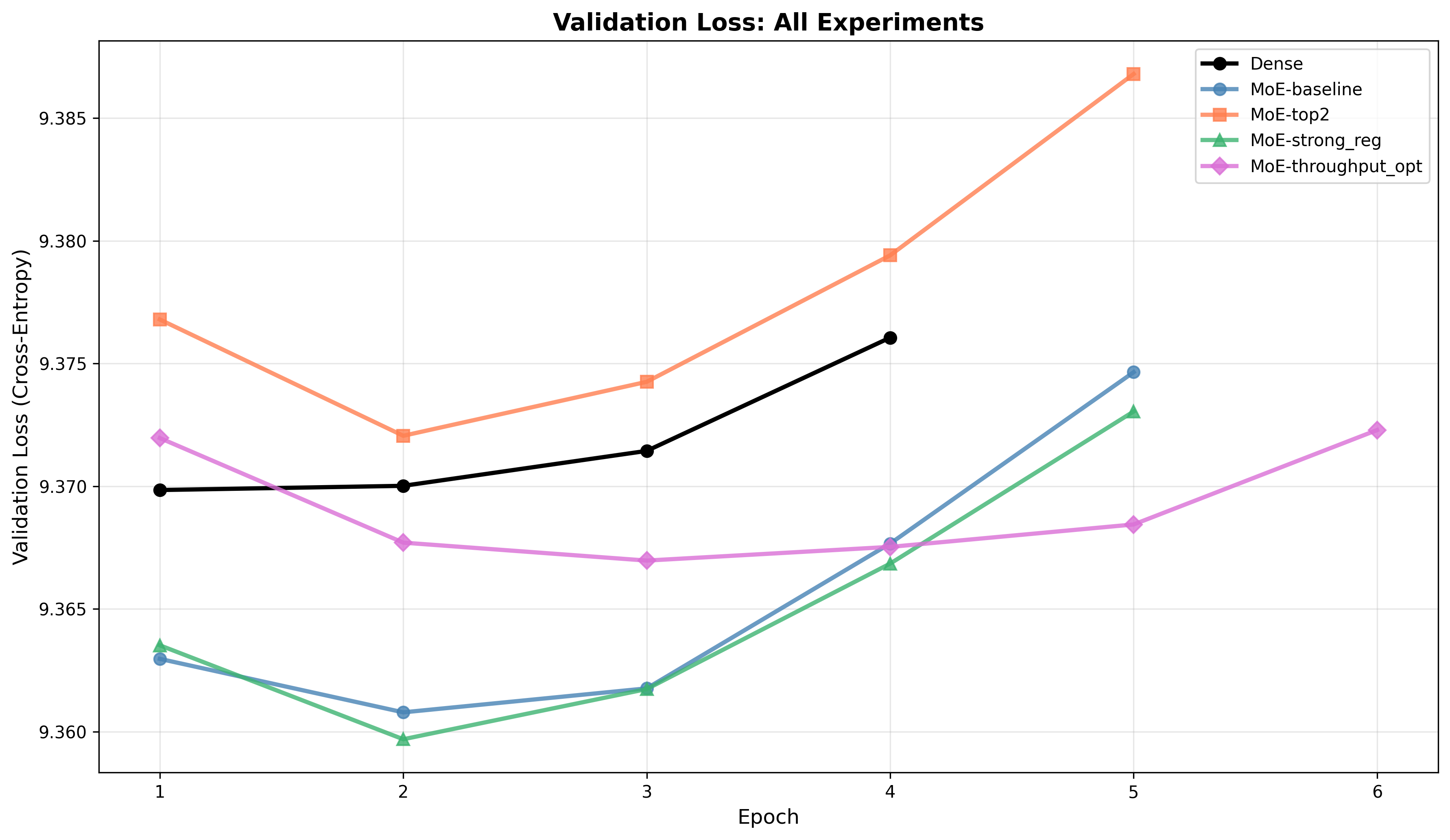
Validation loss: Dense achieves the lowest validation loss (9.3698). MoE variants either match or exceed (worse) the dense validation loss:
MoE-baselineandMoE-strong_regare close to each other and only marginally worse than dense.MoE-top2exhibits the largest gap and a clear upward trend in validation loss after epoch 4, indicating overfitting or gating instability.MoE-throughput_optshows stable validation behavior but does not surpass dense.
-
Interpretation: The MoE configurations give higher representational capacity but require careful gating/regularization and optimization to realize generalization benefits. Without such tuning, larger capacity can overfit or destabilize validation performance.
Throughput and timing breakdown
-
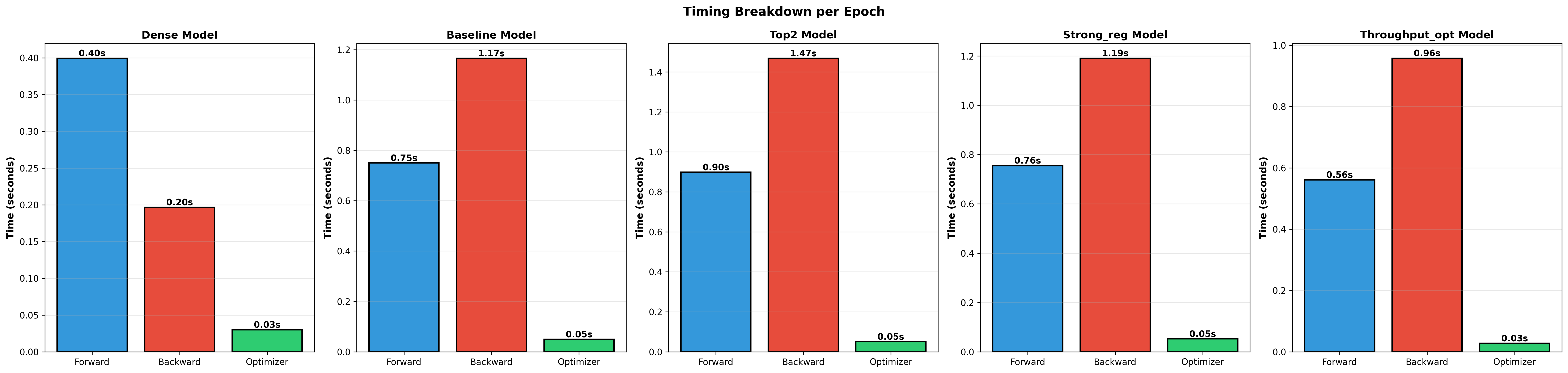
The dominant cost for MoE models is the backward pass. Backward times:
MoE-top2: 1.47 sMoE-baseline: 1.17 sMoE-strong_reg: 1.19 sMoE-throughput_opt: 0.96 s- Dense: 0.20 s
-
throughput_optreduced the backward cost significantly compared with other MoEs, producing the best MoE throughput (54,784 tokens/sec), but still below dense. -
Total per-epoch wall-clock is smallest for dense (0.63s) and largest for
top2(2.42s). -
Interpretation: MoE overheads are chiefly in expert-specific gradient/communication during backward. Optimizations that reduce communication or reduce expert work in backward propagate directly to throughput gains (as
throughput_optdemonstrates).
Expert routing behavior: usage and entropy
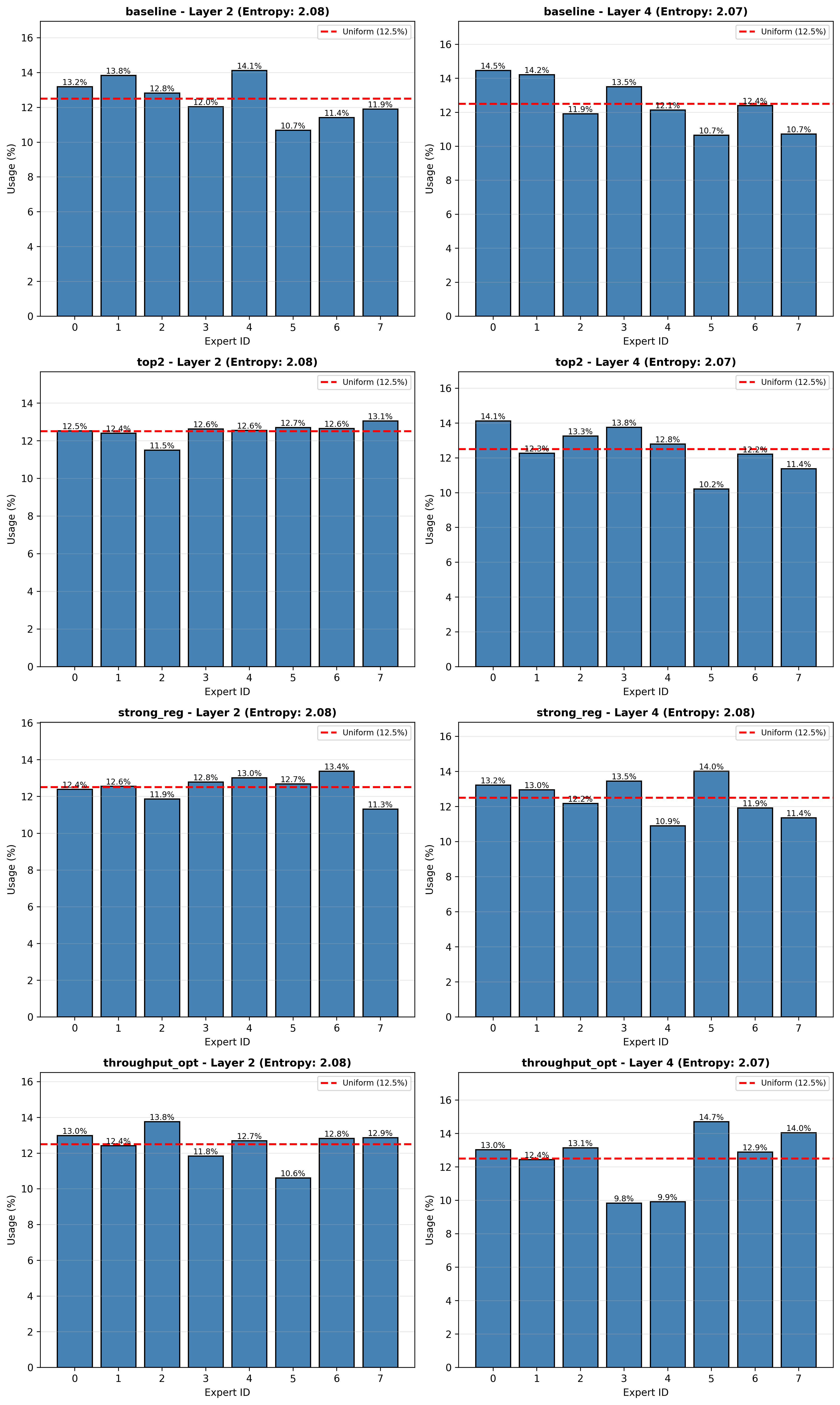
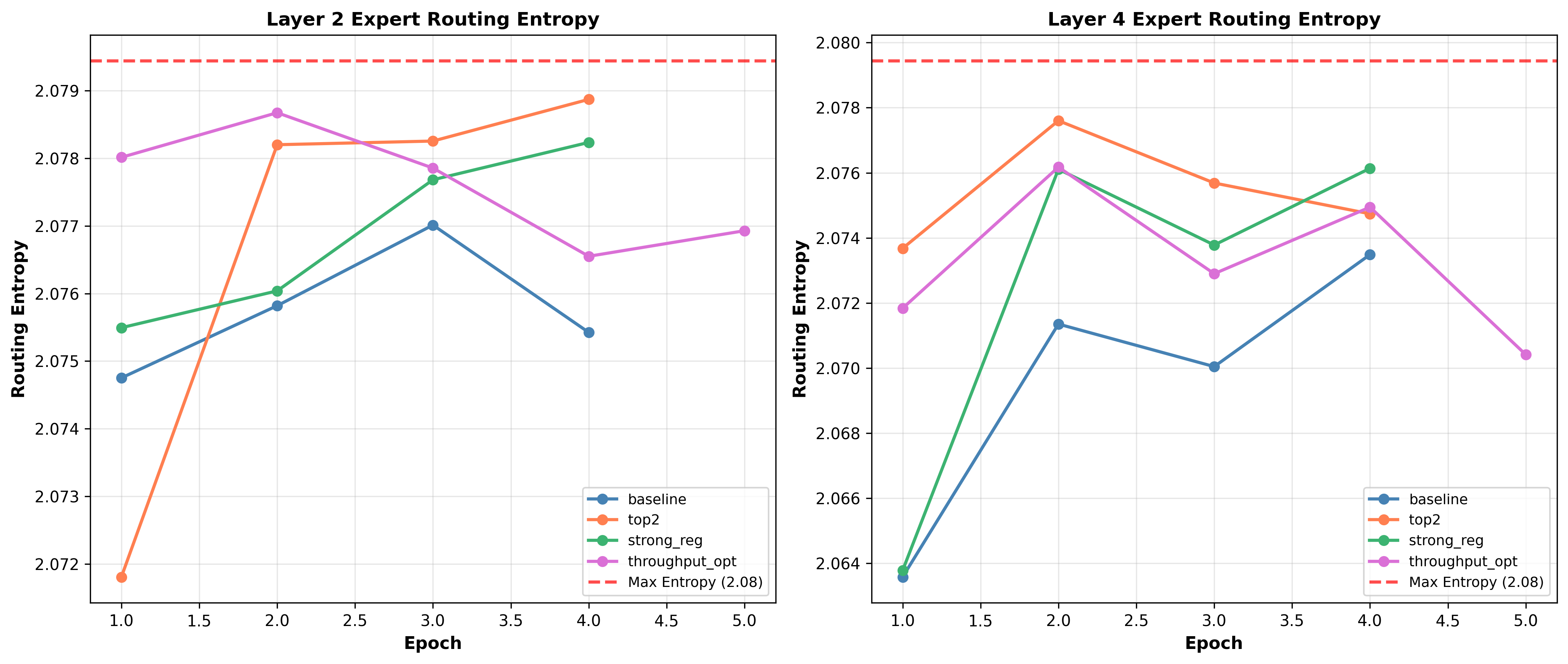
- Entropy: Routing entropy per layer is close to the theoretical maximum (max ≈ 2.08 for 8 experts). That indicates routing is using many experts rather than collapsing to a single expert. Specific observations:
top2layer 2 entropy reaches very close to max early, which matches its aggressive expert usage behavior.- Layer 4 entropies are slightly lower and more variable across experiments.
- Per-expert usage: Usage bars across models and layers show modest deviations from perfect uniformity (uniform = 12.5% for 8 experts). Most experiments show usage within roughly 10.6% to 14.7% per expert. A few spots show underused experts (for example
throughput_optlayer 4 had some experts near 9.8–9.9%). - Interpretation: Routing is generally balanced, but small non-uniformities exist and could cause local specialization or slight load imbalance. Very skewed usage might lead to undertrained experts and affect generalization.
Trade-offs and interpretation
- Dense vs MoE capacity: MoE increases parameter count substantially but this did not translate into better validation loss in these runs. Denser capacity alone is not sufficient to improve generalization.
- Throughput trade-offs: Dense model is faster and achieves better validation performance. For these experiments, MoE costs (especially backward step) made them slower despite higher capacity.
throughput_optshows that MoE overhead can be reduced but not fully eliminated. - MoE-top2 anomaly: The
top2variant fits training data best but generalizes worst. This suggests gating choices (top-2 routing) can increase overfitting risk or cause training instability unless balanced with stronger regularization or gating temperature tuning. - Balancing and entropy: Entropy values close to the max indicate gating is not collapsing, which is good for utilization. However, small routing imbalances can still impact performance. Regularization techniques to encourage balanced loads may help.
Conclusion
Implementation: GitHub
Working through this project gave me a clearer sense of how MoE models behave in practice. I expected the extra capacity from experts to translate quickly into better validation performance, but the results were more nuanced. The dense baseline stayed the most stable and consistent in both speed and generalization, which reinforced the idea that complexity only helps when training dynamics are tuned to support it.
These experiments showed that the dense model remained the strongest, delivering the best validation loss and highest throughput. The MoE variants increased parameter capacity but added meaningful training overhead. The optimized router reduced some of that cost but still lagged behind the dense baseline. The top 2 router trained quickly yet overfit, revealing how sensitive routing is to regularization and tuning. Overall, MoE effectiveness depends on stabilizing routing, maintaining load balance, and improving backward efficiency. Until these factors are refined, the extra capacity offered by experts does not reliably translate into stronger performance.